
Score-Based Causal Discovery with LLMs
Practical Hands-on Techniques for Integrating LLMs Into Causal Discovery Pipelines

This article is also available as a podcast! If you’re on the go or just want to absorb the content in audio format, you can listen to the full episode below 👇 The podcast is also available on Spotify and Apple Podcasts.

Causal questions sit at the heart of applied data science. What drives churn? Why do prices increase? Why did a forecast fail? Correlation alone, no matter how strong, cannot answer these questions.
Causal discovery tackles them by recovering a graph where nodes are variables and edges encode causal influence. The previous article introduced constraint-based methods, which infer this graph through conditional independence tests. They are statistically elegant, but sensitive in practice: errors in early tests propagate, and performance degrades quickly with noisy or high-dimensional data.
Score-based methods take a different approach. Instead of testing independences directly, they assign a score to candidate graphs and search for the structure that best explains the data. This makes them more flexible, more robust to noise, and easier to combine with prior knowledge.
But both approaches face the same limit: multiple graphs can explain the data equally well. Some edges simply cannot be oriented from observations alone. This is where LLMs become interesting. They inject external knowledge about how the world works directly into the search process, helping break ties that statistics alone cannot resolve.
Objective
This article focuses on score-based causal discovery and how LLMs can be integrated into the search process.
After reading this article, you will understand:
How score-based methods differ from constraint-based ones: why framing causal discovery as model selection changes both the search procedure and the kinds of errors the algorithm makes.
Where LLMs can intervene in score-based pipelines: the five integration points, from hard constraints to iterative agentic loops, and which ones are recoverable when the LLM is wrong.
How to pick the right algorithm and LLM integration strategy: comparing priors, post-hoc orientation, and score augmentation on the Adult Census Income dataset, and what each one is worth in practice.
This article is the second part of the series on LLM-augmented causal discovery.
Prerequisites: Basic knowledge of probability and statistics is recommended. The article introduces and explains the main concepts behind score-based causal discovery algorithms.
Tools & libraries:
causallearnfor GES, NOTEARS, and GRaSP.plotlyfor visualization. OpenAI Python SDK for the LLM calls.pandasfor data preparation.
You can find the code here on GitHub.
1. Score-Based Causal Discovery Algorithms
1.1 From Independence Tests to Graph Search
Constraint-based algorithms approached causal discovery as a process of elimination. They start with a dense graph containing every possible connection, then remove edges that fail conditional independence tests. Score-based methods view the problem differently. They treat causal discovery as a model selection problem.
The intuition is straightforward:
Some graphs are too simple and miss real relationships.
Others are too dense and start fitting noise instead of structure.
The best graph is the one that balances explanatory power against complexity.
A score function formalizes this trade-off. The algorithm then searches through the space of possible graphs and keeps the structure with the highest score.
The same running example from the previous article will carry through this section:
S: SmokingT: Tar in the lungsC: Lung cancerA: Age
The true causal structure has three edges. Smoking increases tar accumulation (S → T). Tar increases cancer risk (T → C). Age also affects cancer risk (A → C).
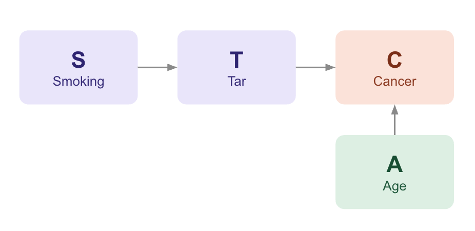
The challenge is to recover this structure from observational data alone.
1.2 What does the score actually measure?
A score function takes a candidate graph and assigns it a single number. Higher means the graph explains the data better.
Every score balances two opposing forces:
Fit: how well the graph explains the observations
Complexity: how many parameters the graph requires
The trade-off is what makes the score useful. Without the complexity term, the algorithm would always prefer the densest possible graph. Adding edges can never make the fit worse. Without the fit term, the algorithm would prefer the empty graph. It has the lowest complexity. The score weighs the two against each other.
The Bayesian Information Criterion (BIC) is the most common score and the default for continuous Gaussian data.
For a single node X_i with parents Pa(X_i), the local BIC score is:
The fit term rewards small residual variance.
Here, σ̂_i² is the residual variance obtained by regressing X_i on its parents. If the parent set explains most of the variation in X_i, the residual variance becomes small.
A small residual variance makes log(σ̂²) more negative.
The leading minus sign turns that into a larger contribution to the score. A good parent set therefore raises the score. A poor parent set leaves large residuals and contributes little.
A good parent set therefore increases the score. A poor parent set leaves large residuals and contributes little.
The complexity term penalizes the parameter count.
The quantity |Pa(X_i)| + 1 is the number of parents, plus an intercept. It counts the regression parameters.More parents mean more parameters to estimate, which increases the risk of overfitting.
The factorlog(n) makes the penalty scale with sample size. As more data becomes available, the algorithm becomes more conservative about adding edges that do not substantially improve fit.
Example Suppose the algorithm evaluates the cancer node
Cwith parents{T, A}. It fits a linear regression of cancer on tar and age, computes the residual variance. It rewards the graph if the variance is small. It penalizes the graph for using three parameters (two slopes plus one intercept). The final score is the balance between explanatory power and model simplicity.
From node scores to graph scores
Once the local score of a node is defined, extending it to the full graph becomes straightforward. BIC computes the score of an entire causal structure by summing the contributions of each node independently:
G: the candidate causal graph
p: the number of variables (nodes) in the graph
X_u: the i-th variable
Pa(X_i): the parent set of X_i
sBIC(X_i,Pa(X_i)): the local BIC score of node X_i given its parents X_i
1.3 How do score-based algorithms search?
Defining a score is only half the problem. The harder part is searching the space of possible graphs.
That space explodes combinatorially. The number of directed acyclic graphs grows super-exponentially with the number of variables. With only 10 nodes, there are already more than 4 × 10¹⁸ possible DAGs. Exhaustive search becomes impossible almost immediately.
Score-based methods therefore rely on approximate search procedures. Different algorithms use different strategies, but most fall into three families:
Greedy combinatorial search
Continuous optimization
Permutation-based search
Each explores graph space differently and makes a different trade-off between scalability, interpretability, and statistical guarantees.
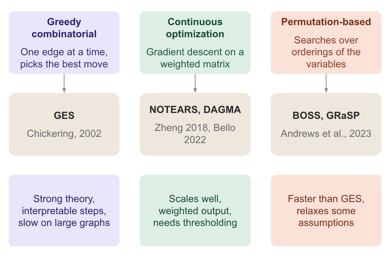
Greedy combinatorial search:
This is the classical approach. The algorithm starts from a simple graph and makes one local change at a time, picking the change that most improves the score.
The canonical algorithm is GES (Greedy Equivalence Search) introduced by Chickering (2002).
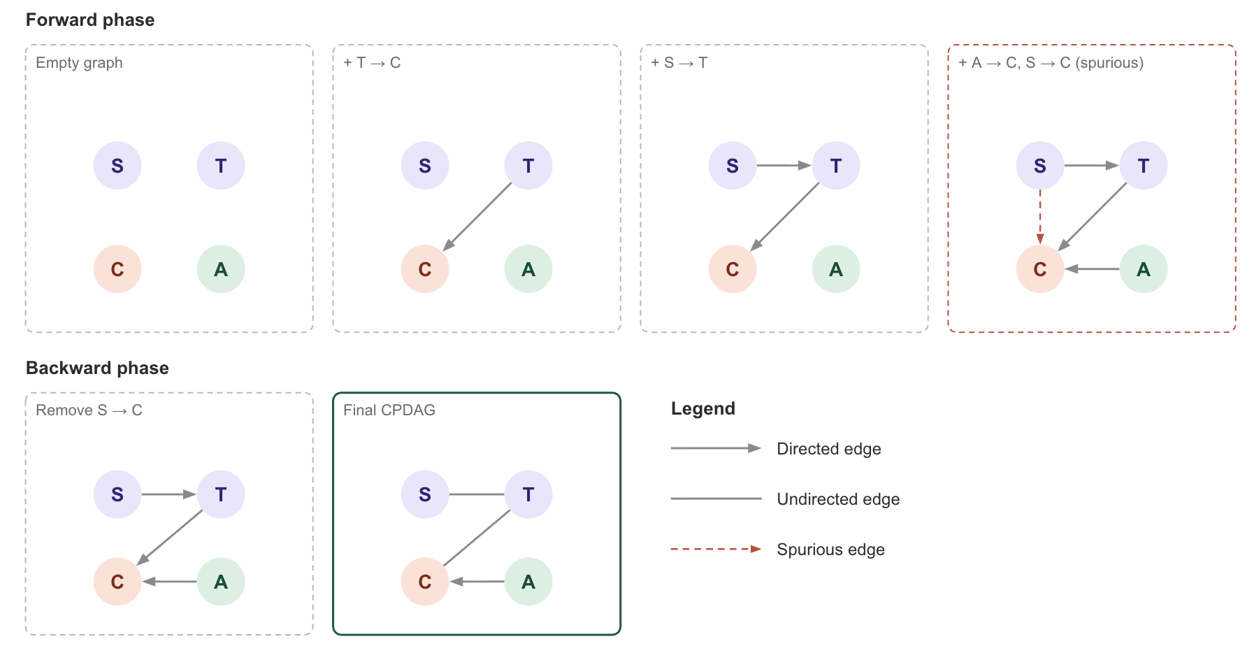
GES operates in two phases:
Forward phase Start from the empty graph and repeatedly add the edge that most improves the score.
Backward phase Remove edges whose deletion improves the score, cleaning up spurious additions introduced during the forward pass.
Note: GES does not search over individual DAGs directly. It searches over Markov equivalence classes. Two graphs that encode the same conditional independences always receive the same score, so evaluating them separately would waste computation.
For the cancer example, GES would add T → C first because tar is the strongest single predictor of cancer in the data. Then S → T. Then A → C. The forward phase ends. The backward phase removes any spurious edges added under finite-sample noise.
The final CPDAG correctly orients T→C and A→C through the v-structure T→C←A, but leaves S—T undirected. The edge S—T cannot be oriented from data alone because the chain S→T→C is statistically equivalent to S←T→C and S←T←C.
Continuous optimization
A more recent family reframes graph search as a continuous optimization problem.
The graph is represented as a weighted adjacency matrix W, where W_ij ≠ 0 means there is an edge from i to j. The algorithm minimizes a continuous loss function over W. The objective is typically a least-squares fit plus a sparsity penalty, subject to a smooth acyclicity constraint:
Each term plays a distinct role.
The fit term
‖X − XW‖²_Fmeasures how well each variable can be reconstructed as a linear combination of the others, weighted byW. A perfect fit meansXW ≈ Xand the residual is zero.The sparsity term
λ₁‖W‖₁is the sum of absolute values of all entries inW. It pushes weak edges toward zero, playing the same role as the BIC complexity penalty. The hyperparameterλ₁controls how aggressively edges get pruned.The acyclicity constraint
h(W) = 0enforces that the resulting graph is a DAG. NOTEARS usesh(W) = tr(e^{W ∘ W}) − d, where∘is the Hadamard product. DAGMA replaces it with a log-determinant formulation that gives a better-behaved optimization landscape and faster convergence.
This formulation was introduced by NOTEARS (Zheng et al., 2018). Later methods such as DAGMA refined the acyclicity constraint to improve optimization stability and scalability.
The key advantage is scalability. Continuous optimization methods handle larger graphs more efficiently than combinatorial search.
The trade-off is interpretability. The output is a weighted matrix rather than a clean graph:
true zero edges often appear as tiny non-zero values
thresholding is required to recover a final DAG
Permutation-based search
Permutation-based search takes a different perspective. Instead of searching directly over graphs, it searches over orderings of the variables.
For example, consider the ordering S,T,A,X. This ordering means that:
S can cause T, A, and C
T can cause A and C
C cannot cause any earlier variable
Once the ordering is fixed, constructing the best graph becomes much simpler because each node can only choose parents from variables that appear before it. The search problem therefore reduces to finding the best ordering rather than the best DAG directly.
Recent methods such as BOSS and GRaSP (Andrews et al., 2023) use this strategy. They often scale better than GES on large graphs and relax some of its theoretical assumptions.
2. Combining LLMs with Score-Based Algorithms
2.1 Why augment score-based search with an LLM?
Score-based methods eventually hit the same wall as constraint-based methods. The limitation is structural and independent of the algorithm itself.
The source of the problem is Markov equivalence. Different causal graphs can encode exactly the same conditional independences.
In the previous article, we saw that constraint-based methods cannot distinguish such graphs because the independence tests return identical results. Score-based methods face the same issue for a different reason: equivalent graphs induce the same likelihood and therefore receive the same score under any criterion derived purely from observational data.
This is not a data scarcity problem that disappears with more observations. More data does not help. A better score function does not help. The missing information simply is not present in the observations.
Resolving the ambiguity requires knowledge that comes from outside the data itself. That is where LLMs become interesting.
2.2 The five roles LLMs can play in score-based methods
Score-based methods offer a much richer integration surface for LLMs than constraint-based methods. The reason is structural: score-based algorithms optimise an explicit numerical objective, and that objective can be modified at several points in the pipeline.
In practice, LLMs can intervene in five distinct ways.
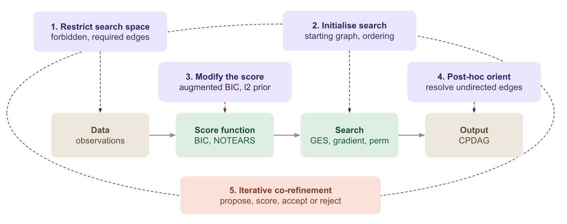
#1. Restrict the search space
The LLM generates hard constraints on which edges are allowed. Forbidden edges are removed from the search space, while required edges are fixed in advance. The score function itself remains unchanged.
This is the classical background-knowledge mechanism already supported by GES [1]. The novelty is that the constraints are produced automatically by an LLM rather than manually specified.
The advantage is simplicity. The downside is rigidity: if the LLM forbids a true edge, the algorithm can never recover it.
Representative work: Hasan and Gani (2023) [3].
#2. Initialise the search
The LLM can also provide a strong starting point:
an initial graph for GES
a variable ordering for permutation-based methods
an adjacency matrix for NOTEARS or DAGMA
The score function stays unchanged, but the optimisation trajectory changes. Since greedy and gradient-based methods are sensitive to initialization, a good starting point can improve both speed and final performance.
Representative work: Vashishtha et al. (2023) [4], Kampani et al. (2024) [5].
#3. Modify the score itself
This is the most natural integration point for score-based methods. Instead of optimizing pure BIC, the algorithm augments the score with an LLM prior:
Each component has a clear role.
s_BIC(G)is the standard log-likelihood-minus-complexity score from section 1.2. The fit-versus-parsimony trade-off is preserved exactly as before.w_ij^LLMis the LLM’s confidence that edgei → jexists, typically a number in[-1, 1]extracted from prompting the model. Positive for endorsed edges, negative for rejected ones, zero for “unknown”. The sum runs over edges actually present in the candidate graphG.λis a hyperparameter controlling how much the LLM influences the score relative to the data. Atλ = 0the algorithm reduces to vanilla BIC. At very largeλthe LLM dominates and the data is ignored. Practical values are tuned on held-out data.
Unlike hard constraints, this approach stays soft: every graph remains searchable, and strong statistical evidence can still override the LLM.
Continuous-optimization methods use the same idea by regularizing the adjacency matrix toward an LLM-generated reference graph [6].
Representative work: Ban et al. (2024) [7], Zhang et al. (2024) [6].
#4. Orient unresolved edges post-hoc
Another strategy leaves the score-based algorithm untouched.
The algorithm first produces a CPDAG, then the LLM is asked to orient only the remaining undirected edges. The LLM therefore intervenes exactly where the data becomes insufficient.
This is safer than modifying the search itself because the LLM cannot invent unsupported edges or remove statistically validated ones.
Representative work: Long et al. (2023) [8].
#5. Wrap the pipeline in an iterative loop
The most recent pattern turns the LLM into an active participant in the search process. Instead of intervening once, the LLM repeatedly proposes modifications to the graph: add an edge, remove an edge, reverse an edge
The score function acts as the verifier. If a modification improves the score, it is kept. Otherwise, it is rejected. The loop continues until the graph stabilizes.
In this setup, the score is no longer just an optimisation objective. It becomes a feedback mechanism guiding an iterative dialogue between the LLM and the data.
This pattern is also the most flexible because it can subsume the previous ones: the LLM can propose constraints, initializations, orientations, or larger restructurings, while the score determines which changes survive.
Representative work: Abdulaal et al. (2024) [9], CauScientist (2026) [10].
2.3 Trade-offs and reliability techniques
The five integration strategies are not equivalent. Their main difference is how recoverable a wrong LLM answer is.
Hard-constraint approaches are the riskiest. If the LLM forbids a true edge, the search can never recover it. Post-hoc orientation has a similar issue: once the LLM commits to an orientation in the final graph, the statistical method cannot revise it afterward.
The other strategies are softer. Poor initializations can be corrected during search. Score augmentation can be overridden by strong statistical evidence. Iterative agentic loops explicitly validate each LLM proposal before accepting it.
This is why recent work increasingly favors post-hoc orientation and iterative verification loops. Long et al. (2023) [8] restrict the LLM to orienting edges only within the Markov equivalence class, while systems such as Causal Modeling Agent [9] and CauScientist [10] route every proposal through a statistical verifier.
Three reliability techniques now appear repeatedly across the literature:
Multi-agent prompting: multiple LLM calls debate or vote on edge orientations to reduce single-prompt bias.
Consistency queries: the same question is asked with shuffled variable orders or rephrased prompts, and only stable answers are retained.
Confidence calibration: the LLM produces confidence scores or multiple samples are aggregated into probabilities, leaving low-confidence edges unresolved.
One caveat remains: LLMs do not learn causality directly. They learn statistical patterns from text. This is why modern methods increasingly treat the LLM as a guide while keeping the data as the final arbiter.
3. Applying LLM-Augmented Score-Based Methods
To illustrate the workflow, we’ll apply causal discovery to the Adult Census Income dataset, the same dataset introduced in the first article of this series. It includes demographic and socioeconomic variables such as age, sex, education, occupation, hours worked, and income.
The dataset is especially useful because it combines three types of variables that causal discovery methods treat very differently:
Immutable factors: age and sex, which are not caused by any other observed variable.
Naturally ordered variables: education precedes occupation, which in turn precedes income. Their temporal ordering is straightforward.
Correlated social features: variables like marital status and relationship, where the causal direction is genuinely unclear.
This makes the Adult dataset a realistic and informative test case. It allows us to examine both the relationships causal discovery algorithms can successfully recover and the situations where they struggle.
The complete code for all experiments in this section is available on GitHub.
3.1. Prior knowledge or LLM guidance: which helps GES more?
GES on its own recovers only what the data statistically supports. Adding external knowledge changes the result, but not always in the same way. Let’s compare three configurations on the same discrete subset to makes those differences more concrete.
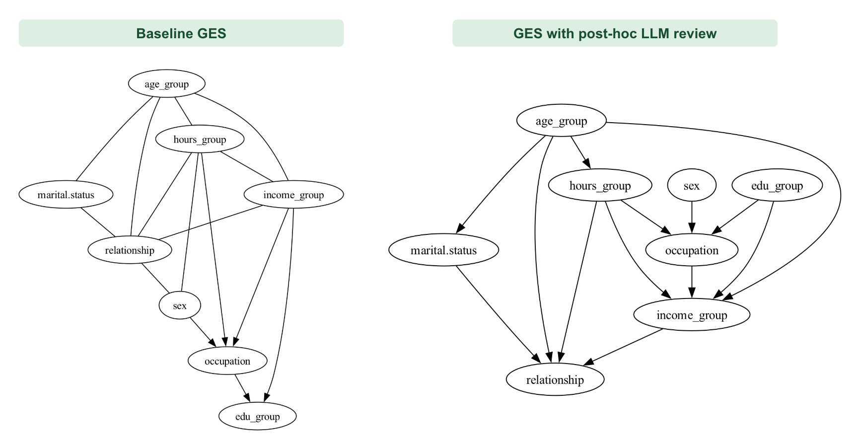
Baseline GES vs. GES with immutability constraints
Baseline GES
The first configuration uses standard GES with the BDeu score and no additional constraints.
BDeu is a Bayesian scoring function designed for discrete data. It measures how well a graph structure explains the observed variable distributions, with a built-in penalty for complexity. It is the standard choice when all variables are categorical.
The result is a CPDAG with a dense demographic core. Most edges involving these variables remain undirected, indicating that the data alone cannot distinguish between several equivalent structures. Only a few edges become oriented, mainly through v-structures around
occupationandedu_group.
Note that a v-structure is a pattern where two non-adjacent variables both point into a common effect (A → C ← B, with no edge between A and B). It is one of the main ways causal discovery algorithms can orient edges directly from observational data. For a more detailed explanation, see the first article in this series.
GES with immutability constraints
The second configuration treats
sexandage_groupas immutable variables, meaning variables that cannot be caused by any other observed feature in the dataset.However, the remaining orientations are still chosen purely by the score. The resulting graph includes edges such as
income_group → edu_groupandincome_group → occupation. Although statistically valid, these directions are difficult to justify semantically since education generally precedes income.
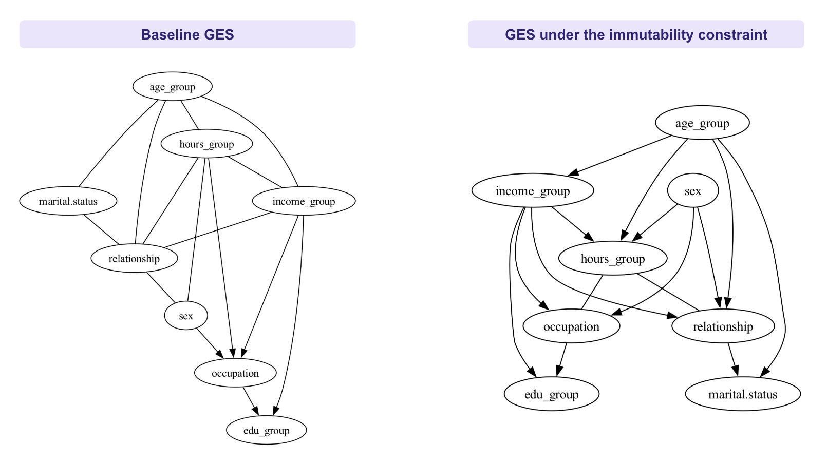
Baseline GES vs. GES with post-hoc LLM review
The final configuration starts from the original CPDAG and asks an LLM to review each edge: keeping, removing, reversing, or orienting it when appropriate. In this version, the problematic orientation is corrected.
The graph now contains edu_group → income_group and occupation → income_group, producing a structure that aligns more naturally with socioeconomic reasoning.
This result looks clean. But it comes with a real risk. The LLM does not see the data. It reasons entirely from variable names and commonsense associations. That means it can orient edges confidently in the wrong direction if the naming is ambiguous, if the domain is unfamiliar, or if the correct causal direction contradicts common intuition.
This illustrates the trade-off introduced in Section 2.3. Hard priors are reliable when the constraint is narrow and uncontroversial, but they provide little guidance for the orientations that matter most. LLM-based review can address those ambiguities by introducing external commonsense knowledge, though at the cost of relying on the model’s judgment.
3.2. Do the three search families converge on the same data structure?
The same dataset can produce noticeably different causal graphs depending on the search strategy.
Running GES, GRaSP, and NOTEARS on Adult Census Income data makes those differences visible: some structures remain stable across methods, while others depend heavily on the assumptions built into the algorithm.
Continuous comparison
Since the standard formulation of NOTEARS assumes linear relationships over continuous variables and is not designed for categorical data, the comparison begins with a continuous subset: age, education.num, capital.gain, capital.loss, and hours.per.week. Raw values are used without transformation, with BIC as the score function for GES and GRaSP. NOTEARS uses its default configuration (λ1 = 0.1, w_threshold = 0.3, L2 loss).
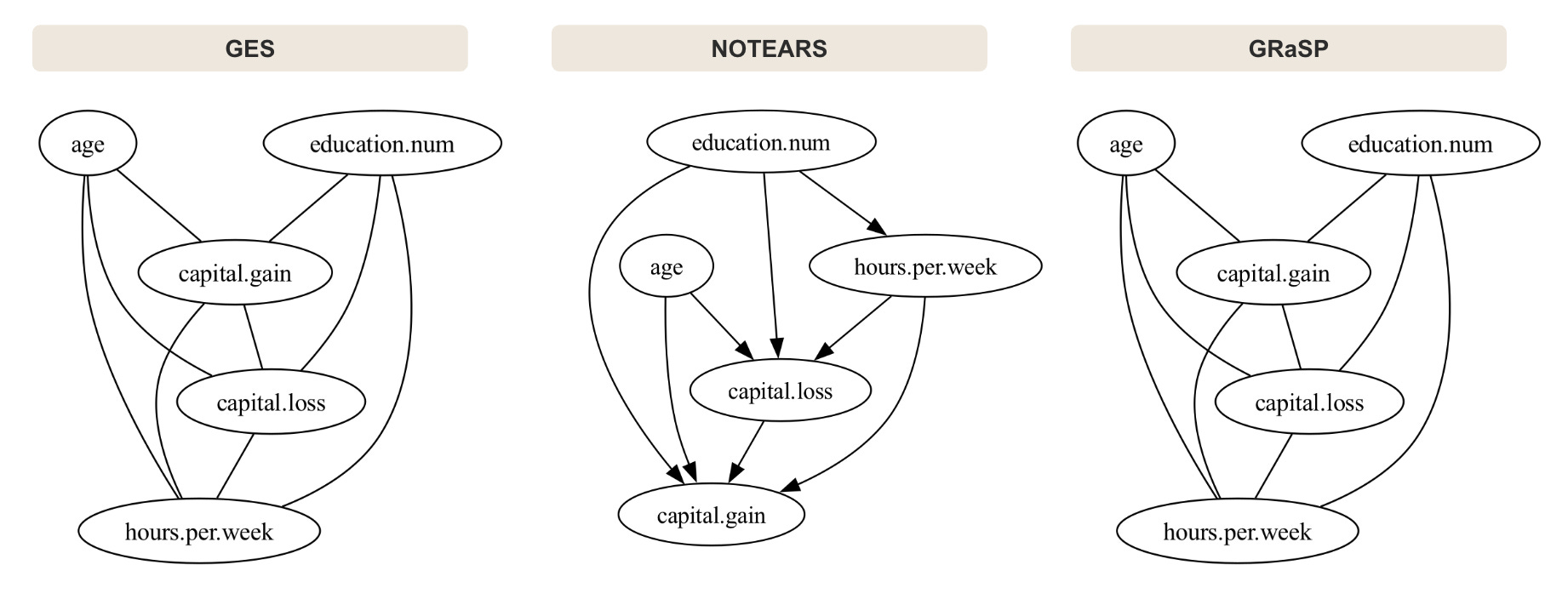
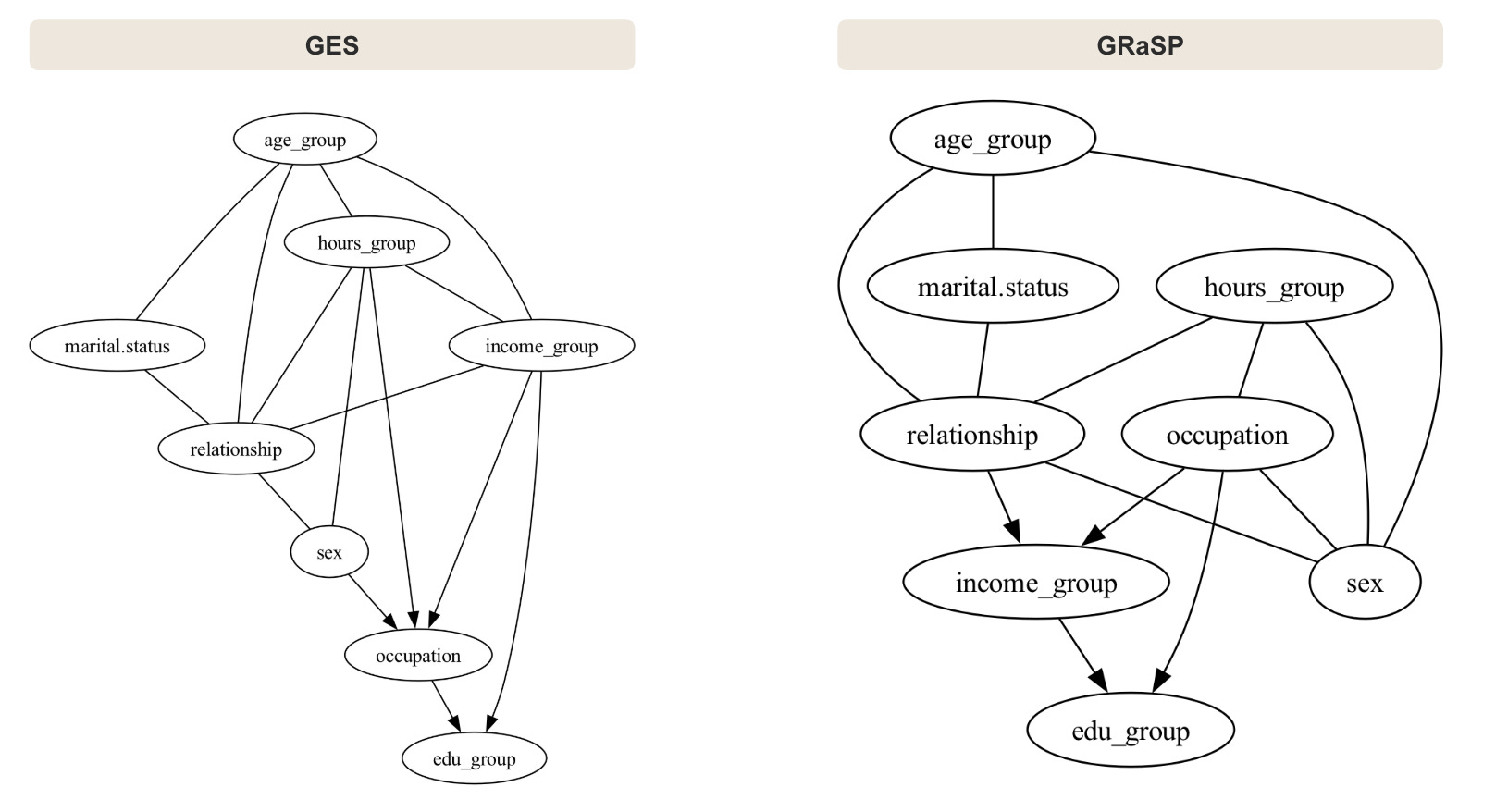
The three methods agree on some broad patterns. education.num, hours.per.week, and the capital variables consistently appear near the center of the graph, suggesting strong statistical dependence between them. However, the orientation of those relationships differs substantially across methods.
GES and GRaSP both return CPDAGs rather than fully directed graphs. Several edges remain undirected because the score cannot distinguish between Markov-equivalent structures. Even though the two algorithms use different search procedures, they recover very similar skeletons and leave many of the same edges unresolved.
NOTEARS behaves differently. Because it optimizes directly over weighted adjacency matrices under an acyclicity constraint, it always returns a fully directed DAG. There is no equivalence-class step. Every retained edge receives a direction, even when the statistical evidence is weak.
Discrete comparison
The discrete comparison includes only GES and GRaSP, using the same categorical subset from the previous section with the BDeu score.
Here, the two methods recover almost identical graphs. The skeletons match closely, and the same edges remain undirected. This agreement is not necessarily evidence that one algorithm is especially accurate. Instead, it reflects a structural limitation of observational causal discovery: under the BDeu score, several graph orientations belong to the same Markov equivalence class, and no search heuristic can resolve them from observational data alone.
Across several runs, variables such as sex sometimes appear in implausible downstream positions. The next section examines how LLM-based penalties discourage these structures.
3.3. How does the LLM penalty influence the scoring function?
This subsection demonstrates the third integration pattern introduced earlier: the LLM modifies the score during the search itself, rather than acting before or after it.
The experiment uses GRaSP. Instead of relying only on BDeu, the score is adjusted with an LLM-derived plausibility penalty. Each possible directed edge receives a score from 0 (“plausible”) to 10 (“implausible”). The prompt also enforces directional consistency: if X → Y is considered highly plausible, then Y → X should receive a much larger penalty.
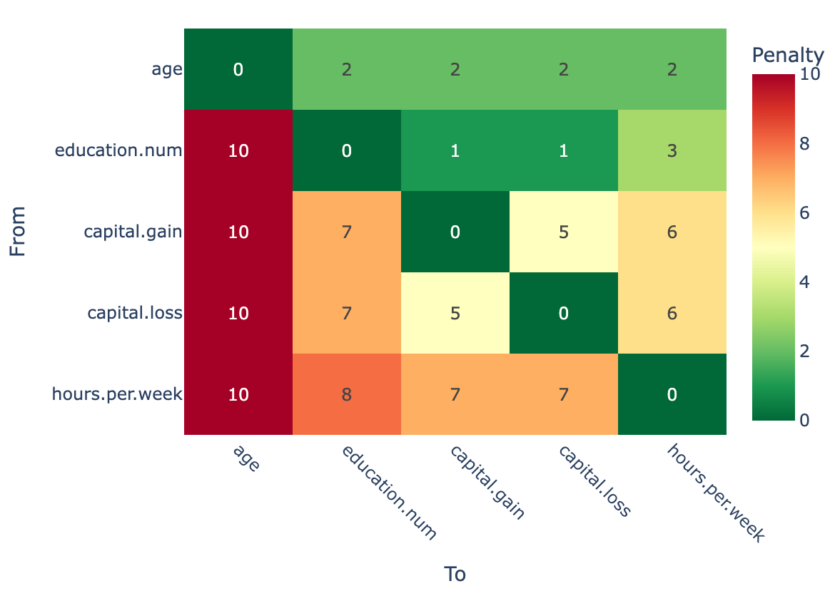
The penalty matrix reveals the type of prior knowledge the LLM injects into the search. Directions consistent with common temporal or socioeconomic ordering receive low penalties, while implausible reversals receive high ones.
For example, edges pointing into age receive the maximum penalty (10), reflecting the assumption that age cannot be caused by other observed variables. Similarly, hours.per.week → education.num is penalized more heavily than education.num → hours.per.week, since education is generally understood to precede working hours rather than result from them.
The matrix is asymmetric by design. Its role is not to remove edges, but to bias the search toward more plausible orientations when several statistically equivalent choices exist.
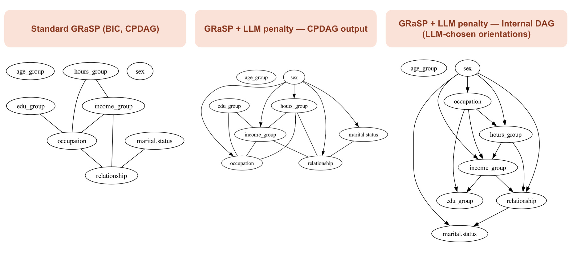
Standard GRaSP: The first graph shows standard GRaSP with pure BDeu scoring and no LLM input. The final output is a CPDAG, meaning that only orientations statistically identifiable from the data survive.
GRaSP with LLM penalties: The second graph applies the LLM-augmented score while still reporting the final CPDAG. The LLM changes which permutation GRaSP prefers internally, but many of those orientations disappear once the graph is collapsed back into a CPDAG. This is the conservative view of the result, the one that reflects only what the observational data can support directly.
Internal DAG before CPDAG collapse: The final graph captures the same LLM-guided run before the CPDAG conversion step. Here, every edge is directed because the permutation search has already committed to a variable ordering. This view exposes the actual influence of the LLM.
The clearest pattern is that the LLM consistently favors commonsense temporal and social orderings. Variables such as age_group and sex move toward the top of the graph, while downstream socioeconomic variables such as income_group, occupation, and marital.status receive incoming edges instead of causing upstream demographic features.
The important point is that the LLM does not invent new dependencies. The skeleton remains largely unchanged. What changes is the orientation selected among statistically equivalent alternatives. The CPDAG intentionally hides most of these choices because the data alone cannot confirm them independently.
Two caveats matter here. First, the LLM-based penalty weight was not tuned. A larger value could dominate the statistical score entirely, while a smaller value might have almost no effect. Second, the prompt evaluates edges independently rather than reasoning over full parent sets, which limits the consistency of the induced graph.
3.4. Do constraint-based and score-based methods recover similar structures?
Finally, let’s compare constraint-based and score-based mehtods. The previous article in this series ran FCI on the same data with the same background knowledge. The two outputs differ in what each algorithm is willing to commit to.
GES with priors returns a CPDAG. Edges are directed when v-structures or constraints force a direction, and undirected otherwise. The algorithm assumes the observed variable set is causally sufficient.
FCI with priors returns a PAG (partial ancestral graph). Edges can carry circle endpoints (
o) to signal uncertainty, or bidirected arrows (↔) to flag a probable latent confounder. FCI does not assume causal sufficiency.
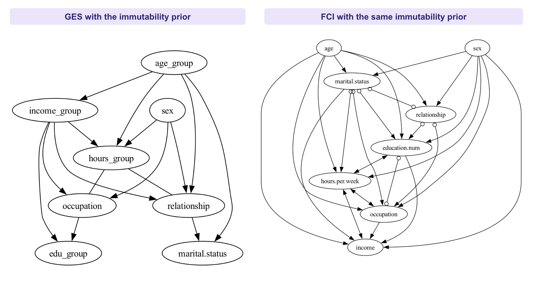
The trade-off is direct. FCI is more honest about what the data cannot decide, especially on a dataset like Adult Censure Income where plausible latent confounders (innate ability, family background, regional labor market) are easy to name.
Neither family is uniformly better. Constraint-based methods such as FCI are preferable when latent confounders are likely and avoiding unjustified causal claims matters more than obtaining a fully oriented graph. Score-based methods are more useful when the goal is to recover a complete DAG for downstream tasks such as causal effect estimation or intervention analysis.
Key Takeaways
✓ Score-based methods reframe causal discovery as model selection: instead of testing independences, they assign a score to candidate graphs and search for the structure that best balances fit and complexity. This makes them more robust to noise than constraint-based methods.
✓ All three search families hit the same identifiability ceiling: GES, GRaSP, and NOTEARS agree on the skeleton but diverge on orientations. Markov-equivalent structures receive the same score. No algorithm can resolve them from observational data alone.
✓ LLMs can intervene at five distinct points in the pipeline: restricting the search space, initializing the search, modifying the score, orienting unresolved edges post-hoc, or wrapping the algorithm in an iterative loop. Each integration point has a different recoverability profile when the LLM is wrong.
✓ Hard constraints are the riskiest LLM integration strategy: a forbidden true edge can never be recovered. Score augmentation and iterative loops are safer because strong statistical evidence can still override the LLM prior.
✓ LLM-based review improves semantic coherence but introduces blind-spot risk: the LLM reasons from variable names alone. It can orient edges confidently in the wrong direction when naming is ambiguous or when the true causal direction contradicts common intuition.
References
[1] David Maxwell Chickering. Optimal Structure Identification With Greedy Search. Journal of Machine Learning Research, 2002. https://www.jmlr.org/papers/v3/chickering02b.html
[2] Xun Zheng, Bryon Aragam, Pradeep Ravikumar, Eric P. Xing. DAGs with NO TEARS: Continuous Optimization for Structure Learning. NeurIPS, 2018. https://arxiv.org/abs/1803.01422
[3] Md. Hasan, Md. O. Gani. LLM-Guided Background Knowledge for Causal Discovery. 2023. https://arxiv.org/abs/2305.12351
[4] Shruti Vashishtha et al. Large Language Models as Priors for Causal Variable Ordering. 2023. https://arxiv.org/abs/2310.15117
[5] Aditya Kampani et al. LLM-DCD: Large Language Model Guided Differentiable Causal Discovery. 2024. https://arxiv.org/abs/2410.21141
[6] Zhang et al. Multi-LLM Regularized Causal Discovery. 2024. https://arxiv.org/abs/2411.17989
[7] Ban et al. Augmenting BIC Scores with Large Language Model Priors for Causal Discovery. 2024. https://arxiv.org/abs/2306.16902
[8] Long et al. Large Language Models as Imperfect Experts for Causal Discovery. 2023. https://arxiv.org/abs/2307.02390
[9] Abdulaal et al. Causal Modeling Agent. ICLR, 2024. https://openreview.net/forum?id=tFVUkS80Lc
[10] CauScientist: Teaching LLMs to Respect Data for Causal Discovery. 2026. https://arxiv.org/abs/2601.13614
[11] Andrews et al. GRaSP and BOSS: Permutation-Based Search for Scalable Causal Discovery. 2023. https://arxiv.org/abs/2310.17009
[12] Bello et al. DAGMA: Learning DAGs via M-Matrices and a Log-Determinant Acyclicity Characterization. NeurIPS, 2022. https://arxiv.org/abs/2209.08037